dbt Migration Framework: 377 Legacy Objects to 51 Models
- SaaS & Tech
TL;DR
A five-month engagement took 377 legacy views, stored procedures, and scheduled queries down to 51 dbt models at first launch, then grew deliberately to 161 models across 7 domains with zero cross-domain breakage. The reduction framework is three moves: kill dead code first — a dependency audit removed roughly 80 objects with no downstream consumers in 90 days — then merge every legacy object producing the same grain into one model with parameterized filtering, then map what remains onto staging, intermediate, and marts. Domain isolation is what made it scale: a schema pair per domain (slv_ and gld_) locked in before the first model and enforced by a generate_schema_name macro override, not by a README convention.
Key takeaway — Most dbt migration guides assume you’re starting from scratch. We started from 377 views, stored procedures, and scheduled queries — some undocumented for years. This post documents the reduction framework: eliminate dead code, consolidate objects at the same grain, isolate domains before scaling. The architecture that emerged took the project from 51 models at launch to 161 across 7 domains with zero cross-domain breakage.
The dbt documentation on project structure is good. It assumes you’re starting from scratch.
Most people aren’t. They’re starting from 377 views, stored procedures, and scheduled queries — some built three years ago, some built last quarter, most undocumented. The guidance for getting from there to a clean three-layer architecture doesn’t exist, or if it does, it lives in conference talks and Slack threads that are hard to find.
Here’s how we did it on a 5-month engagement with a cloud security company. We went from 377 legacy objects to 51 dbt models at first launch, then grew deliberately to 161 models across 7 domains. The reduction was the architecture — and it required a framework for deciding what to keep, what to merge, and what to eliminate.
Quick answer: the reduction framework
If you’re here for the tactical summary:
- Audit everything. Categorize each legacy object by type (view, procedure, query), data domain, and whether anything downstream actually reads it.
- Eliminate dead code first. On most legacy systems, 20–30% of objects are orphaned. Kill them before you plan anything.
- Map remaining objects to the three-layer model. Staging: 1:1 with source tables. Intermediate: joins and business logic. Marts: BI-facing outputs.
- Merge objects that represent the same grain. If three views produce three variants of “metering records for region X,” they become one staging model with a WHERE filter or a macro parameter.
- Isolate domains before scaling. Lock in your schema boundaries (
slv_<domain>/gld_<domain>) before you write your first model. Retrofitting domain isolation on a working project is painful.
That’s the framework. The rest of this post is the detail behind each step and the architecture decisions that determined how we built when the project scaled from 51 to 161 models.
What did the legacy system actually look like?
The cloud security company we worked with ran a large-scale metering and revenue analytics system. Their cloud products reported usage data from 12 regions — some large enough to have dedicated data pipelines, some small enough to share a schema with a WHERE filter. Revenue calculations involved tiered pricing, regional multipliers, account-specific discounts, and a fiscal calendar that doesn’t match ISO quarters.
All of this lived in legacy BI tooling: a mix of database views, transformation logic embedded in dashboard queries, and Jinja macros with hardcoded rate constants — 377 objects in total.
The system produced the right numbers most of the time. The problem was that nobody could explain why. We discovered pricing changes that existed only at the database level with no trace in version control — the kind of accumulated opacity that makes migration necessary in the first place. The full story of what we found is in the revenue analytics migration case study.
How did 377 objects become 51 models?
The first question was what to eliminate.
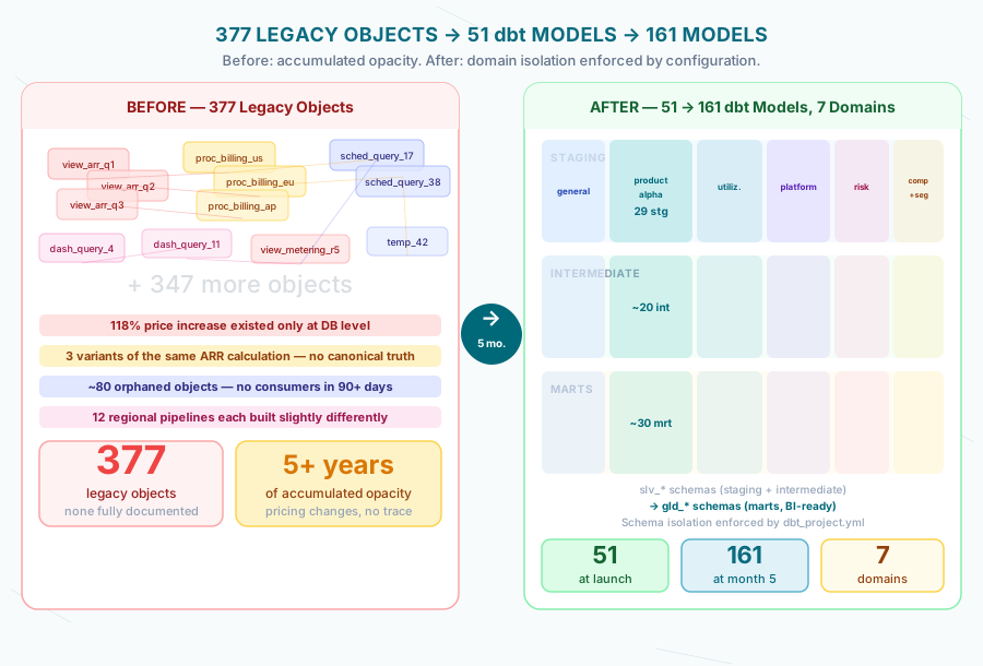
We ran a dependency audit on every legacy object. Anything with no downstream consumers in the past 90 days was a candidate for removal. That pass alone knocked out roughly 80 of the 377 objects — views that had been superseded, exploratory queries left in shared schemas, staging tables from migrations that never completed.
Next: consolidation. Twelve regional pipelines had been built one at a time, each slightly differently. Three ARR calculation variants existed for different reporting contexts. Two dashboards that Finance thought were separate products pulled from the same underlying view with different column aliases.
The consolidation rule: if multiple legacy objects produce the same grain for the same domain, they become one dbt model. Regional variations become parameterized filtering. Reporting variations become mart columns, not separate tables.
After elimination and consolidation, the remaining 51 objects mapped cleanly to a three-layer model:
- 29 staging models — one per source entity, nothing more
- 12 intermediate models — joins, deduplication, business logic
- 10 marts — BI-facing fact and dimension tables
That’s the initial architecture. Domain isolation and materialization strategy were the next decisions that determined whether 51 models could scale to 161 without collapsing under their own weight.
How does domain isolation let a dbt project scale?
The dbt project structure that emerged looks like this:
models:
  metering_dbt_models:
    +persist_docs:
      relation: true
      columns: true

    staging:
      +materialized: view
      +schema: slv_general
      product_alpha:
        +schema: slv_product_alpha
      product_utilization:
        +schema: slv_product_utilization

    intermediate:
      +materialized: view
      +schema: slv_general
      product_alpha:
        +schema: slv_product_alpha
      platform_analytics:
        +schema: slv_product_platform
      risk_analytics:
        +schema: slv_product_risk

    marts:
      +materialized: table
      +schema: gld_general
      product_alpha:
        +schema: gld_product_alpha
      product_utilization:
        +schema: gld_product_utilization
      product_platform:
        +schema: gld_product_platform
      product_risk:
        +schema: gld_product_risk
The key decisions in this structure:
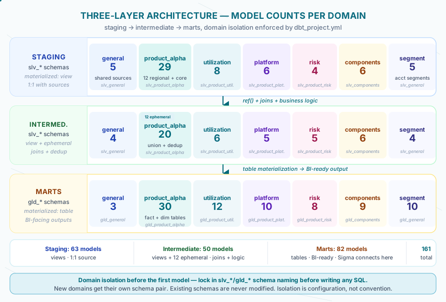
Separate schemas per domain, not per layer. Staging and intermediate for product_alpha both go to slv_product_alpha. Marts for product_alpha go to gld_product_alpha. When the Finance team queries staging data, they know which schema namespace to look in. When a new domain (risk_analytics) was added three months in, it got its own schema pair and didn’t touch anything that existed.
Silver/Gold naming as a contract, not a preference. slv_* means “cleaned, conformed, not yet aggregated.” gld_* means “denormalized, BI-ready, table-materialized.” Snowflake users and Sigma workbooks connect to gld_* only. The naming is enforced by the custom schema macro — not just a convention in a README.
persist_docs at the project root. Every model description flows to Snowflake metadata automatically. This sounds minor until you’re in month four and someone from a domain you didn’t build asks why a column is null in a specific case. The answer is in the DAG viewer.
The key enabler is a generate_schema_name macro override that routes models to the exact schema name specified in dbt_project.yml — not the default dbt behavior that prepends the target schema (turning slv_product_alpha into prod_slv_product_alpha). Without this override, the schema structure falls apart across dev, staging, and prod targets the moment a second developer joins the project.
Where does the “views for everything” default break down?
The default position is “views for everything that isn’t expensive.” That’s the right starting point. The breakdown happens at unions and wide joins.
Ephemeral for union-only models. We had 12 regional staging models that needed to be unioned before deduplication. Making the union model ephemeral means it has zero storage cost and zero schema entry — it’s just SQL that gets inlined into the downstream dedup model at compile time.
{{ config(materialized='ephemeral') }}

select provider, region, customer_id, instance_id, start_date, end_date,
       plan_id, node_count, container_count, /* ... 57 columns total */
       status_code, retry_count
from {{ ref('stg_product_alpha__metering_us_east') }}
union all
select /* same columns */ from {{ ref('stg_product_alpha__metering_us_south') }}
union all
-- 10 more regional refs
57 columns, 12 regions, zero storage overhead.
Views for deduplication, tables for enrichment models that feed 10+ downstream models. The dedup model stays a view — it’s consumed by exactly one downstream model. The account enrichment model is materialized as a table, because every mart in the domain consumes it and computing it once at build time is cheaper than recomputing it for each. The key detail: partition keys must match the legacy system exactly for validation parity, and finding the right partition key took two iterations after we discovered instances reporting to multiple regions simultaneously.
What business logic does a dbt migration surface?
The most valuable part of a dbt migration isn’t the architecture — it’s the business logic that was invisible before. The account enrichment model illustrates this: accounts with no classification record were handled by undocumented date-based rules in the legacy system. Migration exposed them.
{{ config(materialized='table') }}

select
  u.*,
  date_trunc('month', u.start_date)::date as period_month,
  coalesce(a.account_type, '-') as account_type,
  coalesce(a.is_poc, '-') as is_poc,

  case
    when coalesce(a.account_type, '-') = 'INTERNAL' then 'Internal'
    when coalesce(a.account_type, '-') = 'EXTERNAL'
     and coalesce(a.is_poc, '-') = 'Yes' then 'External POC'
    when coalesce(a.account_type, '-') = 'EXTERNAL'
     and coalesce(a.is_poc, '-') = 'No' then 'External Upside'

    -- Orphan accounts: match legacy date-based treatment.
    -- Pre-2023 ELA period (Jul 2021 - Dec 2022): treat orphans as External POC.
    when date_trunc('month', u.start_date) >= '2021-07-01'
     and date_trunc('month', u.start_date) < '2023-01-01'
      then 'External POC'

    when coalesce(a.account_type, '-') = '-' then 'Unknown'
    else 'Unknown'
  end as account_segment

from filtered_usage u
left join account_inventory a
  on u.account_id = a.account_id
  and u.plan_name = a.plan_name
  and date_trunc('month', u.start_date)::date = a.period
This is one of 15 bugs we found and fixed during the migration. The full reconciliation methodology is in the revenue analytics migration case study.
How did the project scale from 51 to 161 models?
The architecture scaled by domain addition, not by model sprawl.
| Phase | Models | Domains added |
|---|---|---|
| Phase 1 (month 1) | ~34 | Core metering (product_alpha) |
| Phase 2 (month 2) | ~50 | Product utilization, business data |
| Phase 3 (month 3) | ~90 | FY27 pricing, v2 models, dimensions |
| Phase 4 (months 4–5) | 161 | Platform, risk, components, segment |
Each new domain got its own schema pair and its own folder in models/staging/, models/intermediate/, and models/marts/. No existing models were modified. New domains couldn’t break old ones because schema isolation is structural, not conventional.
For major logic changes — specifically the FY27 pricing rebuild — we ran v1 and v2 models in parallel, comparing outputs row by row before deprecating v1. That sprint is covered in the FY27 pricing post.
The materialization breakdown at 161 models: 29 staging (views), 50 intermediate (views + ephemeral), 82 marts (tables + dimension views). The ratio of roughly 1:1.7:2.8 across the three layers is a reasonable prior for a multi-domain metering system.
377 objects became 51 because most of them didn’t need to exist. The ones that did map cleanly to three layers — and once domain isolation is in place, adding the other 110 models takes care of itself.
Domain isolation is a core pattern in our Unified Data Foundations approach. The full story of how this migration grew from one product domain to seven is in Scope Growth Done Right.
Every number from this migration — scope, timeline, defect counts, validated variance, and Year 1 return — is collected as a citable reference card in the dbt migration benchmark.
If your dbt project inherited years of legacy objects and you’re not sure what to keep, we’ve built the reduction framework. Start with an architecture review.
Frequently asked questions
How do you reduce 377 legacy BI objects to 51 dbt models?
Three steps: classify each object as keep, merge, or kill against the business questions actually being asked; consolidate similar logic into reusable macros and shared models; and drop the 20–30% of objects nobody has queried in the last 90 days. The reduction comes out of duplication and dead weight, not lost reporting coverage.
What is a three-layer dbt architecture and why does it scale?
Staging holds 1:1 source mappings, typed and renamed; intermediate holds business logic and cross-source joins; marts hold the final business-facing models grouped by domain. The split lets each layer change for a different reason — source schema changes, business logic shifts, reporting needs — which is what absorbed growth from 51 to 161 models without collapsing.
How do you keep a dbt project from breaking as new domains are added?
Give each domain its own schema pair and its own folder under staging, intermediate, and marts, then enforce the routing in dbt_project.yml so a new model lands in the right schema regardless of what anyone writes in the model config. Across four phases and 110 added models, no existing models were modified and no new domain broke an old one, because schema isolation is structural rather than conventional.
How do you decide what belongs in intermediate versus marts?
Intermediate models can be consumed by other intermediate models or by marts, but they never contain columns designed for BI display — a formatted_revenue column or a display label belongs in a mart. The practical test: if a mart could consume the model without any further joins, it is probably a mart; if it still needs joins to be useful, it is intermediate.
When does the three-layer dbt model break down?
It struggles with cyclical dependencies — cases where domain A enriches domain B and domain B classifies domain A. We hit a version of this with account segments derived from the account inventory domain feeding into the metering revenue domain, and the fix was making account segment derivation self-contained within a single intermediate model rather than a cross-domain dependency. Wanting a ref() that crosses domain boundaries at the staging layer usually means your domain boundaries are wrong.
What's the right number of dbt models for a project this size?
161 models for 7 domains across 5 months is on the higher end, but domain count drove it more than complexity — the core metering domain alone accounts for roughly 79 models, since it had 12 regional pipelines and 31 pricing macros. A single-domain project of similar complexity would land somewhere in the 60–80 model range. Sitting at 200+ models on a single domain usually means intermediate models are doing work that should be split into smaller, more focused ones.
How do you handle dev/prod schema separation without dbt Cloud?
Per-developer databases plus a validate_dev_target macro that blocks production runs unless the CI flag is set, with each developer's schema named dev_<name>_slv_product_alpha rather than slv_product_alpha and the generate_schema_name macro handling the routing. Because Snowflake-native dbt has no local development workflow — every model test requires a push and execution in Snowflake — per-developer databases matter more, not less.
How do you prevent schema drift as new engineers join a dbt project?
Two mechanisms. dbt_project.yml enforces schema routing at the configuration level, so a new model in models/staging/product_alpha/ lands in slv_product_alpha regardless of what anyone writes in the model config. And CLAUDE.md, the project's AI instruction file, carries the naming conventions and schema rules explicitly, so any session that starts by reading it has the conventions before touching code — covering human drift and AI drift in the same mechanism.